Spreadsheets get a bad rap for being hard to read. Making spreadsheets user friendly is all about adding a bit of formatting—taking basic steps like adding column headers, adjusting your alignment, and using the right color in your spreadsheets.
Formatting is a must, but conditional formatting is even more powerful. Conditional formatting changes how a cell appears, based upon what's inside the cell.

In the screenshot above, you can see the power of conditional formatting. I've setup a very basic rule that turns the background of a cell with a positive value green, while a negative value will turn red.The only thing that changes is the background color based on the value.
Other examples of conditional formatting could include:
- Putting all negative numbers in a list of data in red.
- Creating data bars to give a visual representation of the largest and smallest items in your data set.
- Using icons to indicate the highest and lowest values in a list of data.

When you write conditional formatting, the formatting adjusts to what's in the cell. In this tutorial, you'll find out how easy it is to use conditional formatting in Excel.
How to Apply Conditional Formatting in Excel (Watch & Learn)
In this video, I'll walk you through some of the easiest ways to apply conditional formatting. You'll get an over-the-shoulder look at how I use conditional formatting in Excel to highlight important data.
The rest of this tutorial will focus on adding conditional formats to your spreadsheets. Read on to find out how you can use them in your own spreadsheets.
1. Using Built-in Conditional Formatting
This tutorial includes an example spreadsheet that you can download for free and use for the steps below.
Spreadsheets can be overwhelming at times. The good news is that conditional formatting in Excel is easy to get started with thanks to Excel's built-in styles.
We're going to take a look at Excel's built-in styles for conditional formatting. For each of these styles, you can apply them by highlighting the list of data you want to format, and then finding the Conditional Formatting button on the Home tab of the ribbon.
Once you've opened the Excel conditional formatting menu, choose one of the options to begin applying conditional formatting.
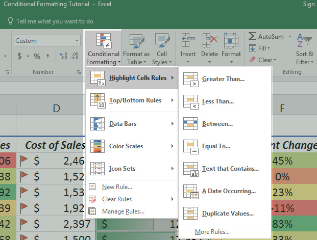
Highlight Cells
Choosing the highlight cells option allows you to conditionally format cells on a variety of factors. Click on Conditional Formatting and choose one of the options from the Highlight Cells Rules menu to get started with conditional formatting.

Think of these options as presets for conditional formatting. Here's how each work:
-
Greater Than - Format cells greater than a value that you set.
- Less Than - Format cells lower than a value you set.
- Between - Give conditional formatting to a range of values, and highlight cells between those values.
- Equal To - Format a cell when it is exactly equal to a value you set.
- Text that Contains - Format cells that contain strings of text.
- A Date Occurring - Conditional formatting based upon the date in a cell.
- Duplicate Values - Quick conditional formats for a list of data with duplicates.
Let's look at an example. I'll choose Greater Than for my example. Then, I'll set a value in the pop up window. In the screenshot below, I set my value to be $22,000, and used the "Green fill..." option.

As you can see, Excel applied conditional formatting in the preview, and all values greater than $22,000 were highlighted in green.
This menu is a great way to customize your conditional formatting rules. You can easily build rules for how to format your cells by starting with the "Highlight Cells" option.
Apply Top/Bottom Rules
Another great way to set Excel conditional formatting is with the Top/Bottom Rules option. You can easily choose to highlight the top and bottom 10 items in a list, or apply another option.
Click on the Conditional Formatting option, choose the Top/Bottom Rules panel, and then choose one of the formatting options shown.

In my case, I'll choose the Above Average option to highlight all of the sales amounts that are above the average in the set.
The pop up window is very similar to the prior example, and we'll select Green Fill... from the dropdown.

Notice in the screenshot above that Excel automatically highlights in green any of the cells in green.
2. Use Built-In Styles in Excel
The options we've looked at so far require giving Excel some rules. If you want the fastest way to add conditional formatting, try out some of the options below.
Work With Data Bars
One of the quickest ways to add meaning to your spreadsheet is to choose the data bars option. Data bars will place bars inside of cells that represent the "size" of the data in your list.

To apply a data bar conditional format, highlight your data first. Then, find the Data Bars option and choose from one of the gradient or solid fill options.
The screenshot below shows the power of data bars to illustrate data. In the January 2017 column, the green gradient bars correspond in length to the amount. The lowest amounts have the shortest bars, while higher amounts have longer bars.

Data bars are a great illustration of the power of conditional formatting in Excel. Notice how much easier it is to find the largest amounts than the February column, just by scanning the lengths of the bars.
Apply Color Scales
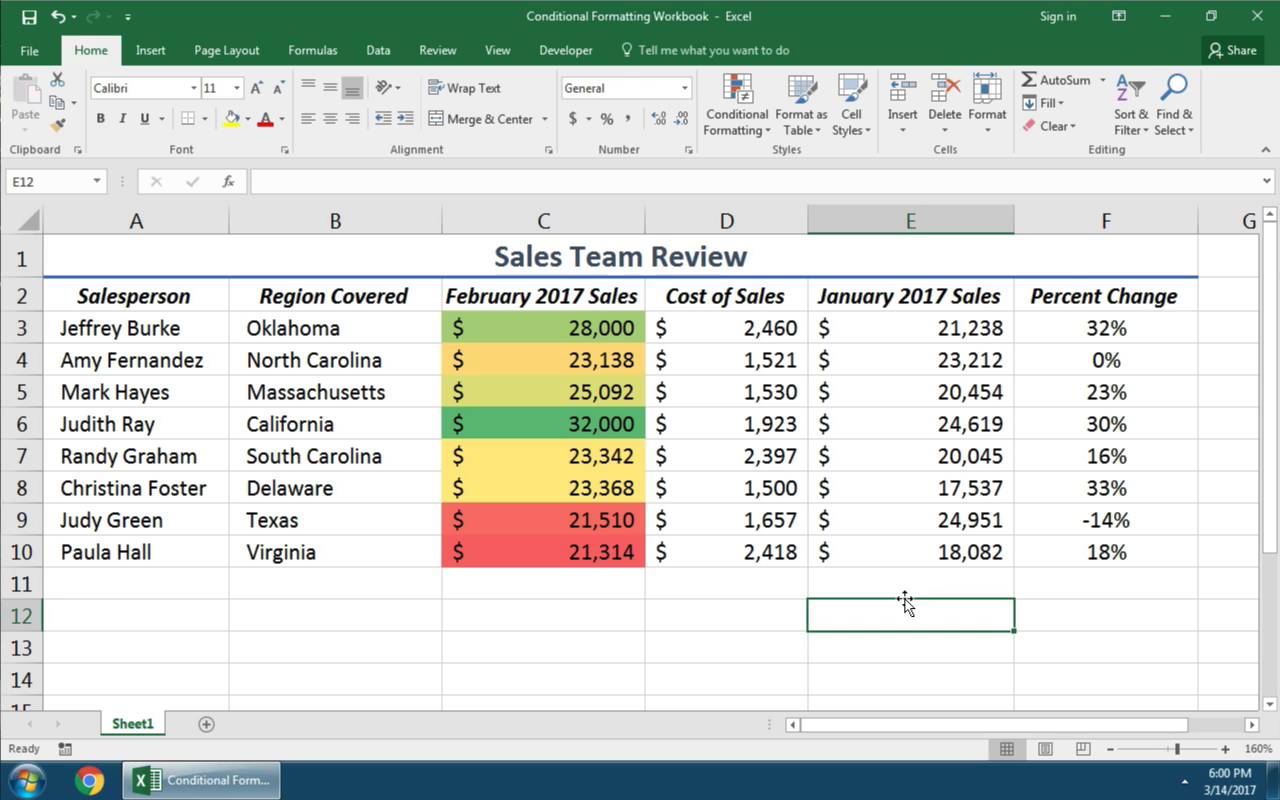
Color scales really draw attention to the highest and lowest values in a list of data. After you've highlighted your data, return to the Conditional Formatting option, and choose one of the options from the Color Scales menu.

The color scales in the thumbnails represent the colors that will be applied to your data. I'll choose the first icon in the list, and you can check out the results below:

In the example above, the best sales result has a dark green background, while the lowest value is in red. All of the other values are in shades of yellow and green, to represent the salesperson's performance.
The color scales option has a variety of Excel conditional formatting rules. Try out several of the other thumbnails to apply other colors to your data.
Add Icon Sets
Icon sets are another great way to add some extra style to your spreadsheet. In my example, I'm going to highlight my data, and choose some arrows from the conditional formatting options.
The icon sets include arrows to show changes in data, as well as other icons like flags and bars to show data right inside of the cell.
In the data below, I have a percent change column to show how the salesperson performed versus the prior month. This is a great way to visually represent your data.
Each of these built-in icon styles is designed to help you make judgments about your data by quickly glancing at it.
All of these conditional formats adapt when the data changes. If the sales figures changed, Excel would automatically change the icon accordingly.
Usually, I start with one of the built-in styles and modify it to my liking. It's much easier to use a built in conditional formatting option and tweak it, instead of writing your own from scratch.
Recap and Keep Learning
This tutorial covered Excel conditional formatting. You learned how to add styles to your cells that change dynamically based upon what's inside of the cell.
Here's the thing: using formatting makes your spreadsheets easier to read. But using conditional formatting in Excel helps you add insight directly to your cells. It allows you to glance through your data and understand it rapidly.
Here are more great tutorials to help you level up your Excel skills:
- If you'd like a more basic Excel tutorial to get started, check out the beginner's tutorial How to Make a Basic Formula in Excel.
- Learn more about formatting with How to Use the Excel Format Painter in 60 Seconds.
- This tutorial covered conditional formatting, which changes a cell's appearance based upon the contents. We can also use conditions to change the data in a cell, with How to Use Simple IF Statements in Excel.
How are you using conditional formatting? What are your favorite styles to apply to a cell and how do you use it? Let me know in the comments.
 By
By