

PivotTables can transform your career. If you work in an office environment and know how to use Excel, you can build out reports and files to help everyone understand their data.
A slicer is a PivotTable feature that makes reports interactive. Instead of using the filter buttons inside the PivotTable, a slicer adds point and click options to filter your data.

Imagine using a slicer to filter your data for a specific year. You have a slicer box with each year that's in the data, like "2016" and "2017." To see just the 2016 data, you can click on it in a slicer box to filter for that data in the PivotTable.
This makes reports interactive and user-friendly. Hand off a PivotTable with slicers to a co-worker and they won't have to come back to you each time they need a different report.
In this tutorial, you'll learn how to insert Excel slicers and customize them to make it easy to work with PivotTables.
Background: What's a PivotTable?
Basically, a PivotTable is a drag and drop tool to build reports in Excel. You can take a large spreadsheet of data and turn it into meaningful summaries in just a few minutes with a well-built PivotTable.

What Is a Slicer in Excel?
Slicers make it even easier to work with PivotTables. You can create simple buttons for your user to click on to filter the data. They make it much more user-friendly to work with PivotTables.
If you want to get started with PivotTables, check out some of the tutorials below before you dive into the rest of this tutorial.
 How To Make Use of 5 Advanced Excel Pivot Table Techniques
 How to Create Your First PivotTable in Microsoft Excel
Now, let's dive into creating and customizing slicers in Excel.
How to Quickly Insert Slicers into Excel PivotTables (Watch & Learn)
In this quick screencast, I'll show you how to add slicers into your PivotTable and then customize them. These slicers will help you filter and refine the data that shows in your PivotTable.
Keep reading to find out more about how to use slicers in Excel to your advantage:
Add Your First Excel Slicer
To get started with slicers, start off by clicking inside of a PivotTable. On Excel's ribbon, find the PivotTable Tools section and click on Analyze.
Now, look for the menu option labeled Insert Slicer. Click on it to open up a new menu to select your slicers.

On the new menu that pops up, you'll have checkboxes for each of the fields that are in your PivotTable. Check the boxes for the slicers you want to add.
Once you press OK, you'll see a box for each of the filters. You can drag and drop these slicer windows to other areas in the spreadsheet.

That's it! You've inserted a slicer for fields. You can now point and click to filter your data. Let's learn more about how to use and customize filters.
How to Use Slicers in Excel
This part of the tutorial will focus on how to use slicers to analyze your data. Remember: slicers are simply user-friendly filter buttons.
Once you have a slicer inside of your spreadsheet, you can simply click on one of the boxes inside the slicer to filter your data. You'll see the data in the PivotTable change as you click on a slicer.

As you click on the slicer buttons, the PivotTable updates to only show data that matches your filter settings.
You can use a slicer to filter data that isn't showing in the table. Basically, what that means is that even if you don't see "year" as a row or column in the PivotTable, you can still have a "Year" slicer that changes the data that shows in the Pivot.
Let's say that you want to select multiple items in a Slicer. You can hold the Control key on your keyboard and click on multiple items in the Slicer so that the Pivot filters for all of the items you've selected.

Finally, slicers stack. After you click on a button inside of a slicer, you'll see other slicer options grey out. This means that the first filter you applied has "knocked out" other options, making them unavailable to click on.

To clear your slicer settings, you can always click the small icon in the upper right corner, which is a filter button with a small red X. This will undo all filters that you've applied with the slicer.
Advanced Excel Slicer Options
Let's learn a few more techniques to really enhance how you can work with slicers. To work with most of these options, make sure that you have a slicer selected and click on the Slicer Tools > Options menu on the ribbon to make these settings visible.

Styling Slicers in Excel
You can easily change the color of slicers to make them stand out. In the Slicer Styles section of the ribbon, you can simply click on one of the other color thumbnails to change the style of the slicer.

Multi-Select
Remember how you learned to hold control on the keyboard to multi-select items in a slicer? There's another way to make this option work.
Near the upper right of each slicer, there's a checkbox button that you can click on. When this option is turned on, you can multi-select and toggle options off or on by clicking on them.

This is a great option if you're sending the PivotTable to other users to work with.
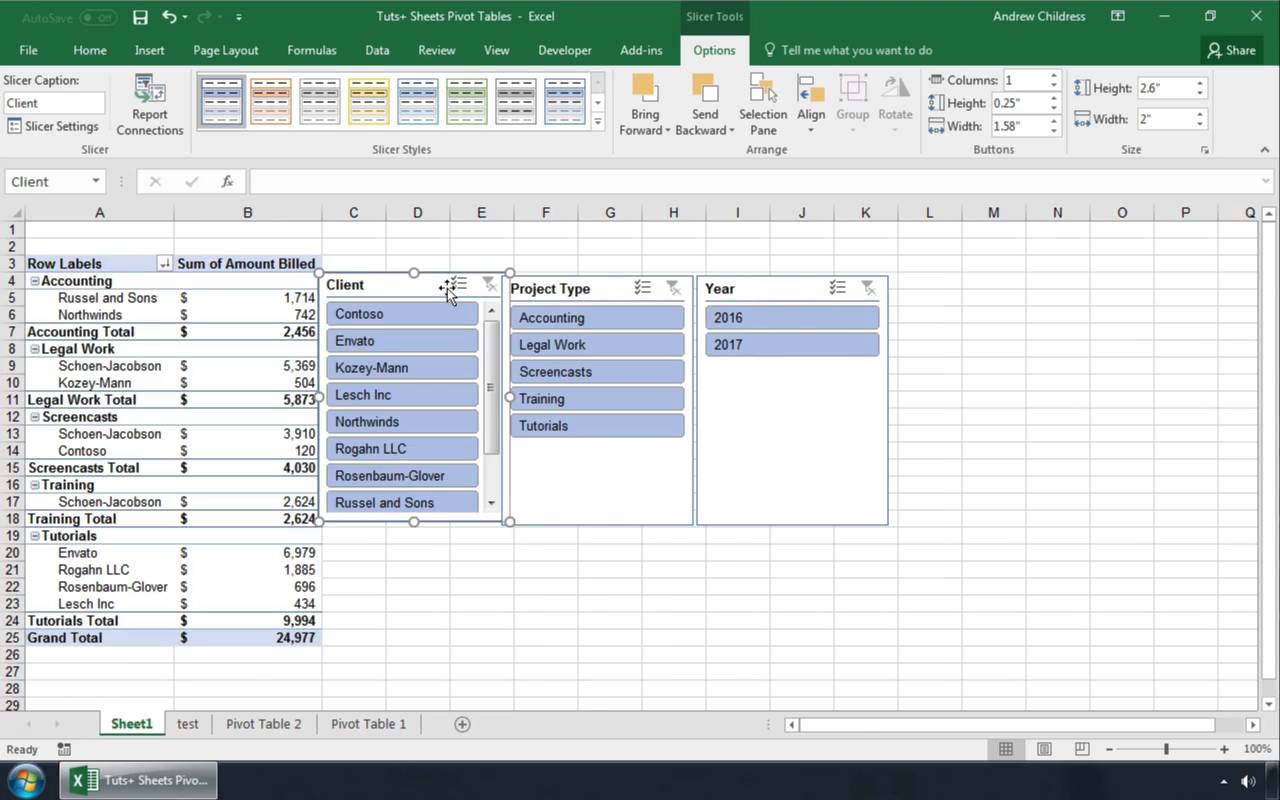
Multiple Columns in the Slicer
If you have many options inside the slicer, they may not all fit within the window. Excel will add a scrollbar. However, it can be cumbersome to scroll up and down within that window.
The solution is to have multiple columns of buttons in the slicer. With the slicer selected, find the Buttons section of options on the Slicer Tools > Options menu. In the columns menu, change the number so that more columns show inside the slicer.

Excel Slicers Connected to Multiple Tables
Here's one of my favorite tricks for using slicers across multiple Excel PivotTables. If you have multiple PivotTables connected to the same data, it helps to connect a slicer to control multiple tables. Click on a filter in a slicer and all of the PivotTables will update in lockstep.
To connect a slicer to multiple Pivots, click on a Slicer box and choose Slicer Tools > Options on Excel's ribbon. Then, click on Report Connections to open up the settings.
This window controls the PivotTables that the slicer controls. Simply check the boxes for the Pivots you want the slicer to connect to, and press OK.

Now, the slicer will control multiple PivotTables. You don't have to click on multiple slicers to keep those PivotTables in sync. Imagine using the first sheet of your Excel workbook with all of the slicers to setup your next report, with all of the tables updating together.
Recap and Learn More Excel Data Tools
I can't say enough about the power of slicers. PivotTables are a great start to analyzing your data better, and slicers make them easy to hand off to other users for easy filtering. Instead of generating multiple reports, let the viewer create different views using slicers.
Here are some additional resources to help you work with slicers and PivotTables in Microsoft Excel:
 How to Use PivotTables to Analyze Your Excel Data
 How To Make & Use Tables In Microsoft Excel (Like a Pro)
 How to Link Your Data in Excel Workbooks Together
Any questions? Feel free to let me know in the comments section below if you need any ideas on how to use slicers in Excel PivotTables.
 By
By


