If you need to work with percentages, you’ll be happy to know that Excel has tools to make your life easier. Excel percentage formulas are a great tool for perfect, proportional calculations every time.

As an example, you can use Excel to track changes in track business results each month. Whether it’s rising costs or percentage sales changes, you want to keep on top of your key business figures. With an Excel percentage formula, you can do this with ease.
In this tutorial, learn how to calculate percentages in Excel with step-by-step workflows. Let’s look at some Excel percentage formulas, functions, and tips. To do that, we'll be using a sheet of business expenses and a sheet of school grades.
You’ll walk away with the techniques needed to work with percentages in Excel right away! Let's learn how to calculate a percent increase in Excel and so much more.
How to Calculate Percentages in Excel (Quickstart Guide)
Watch the complete tutorial screencast, or work through the step-by-step written version below. First, download the source files for free: Excel percentages worksheets. We'll use them to work through the tutorial exercises.
Want to learn more options for how to calculate a percent increase in Excel? Plus, how to calculate percentage in Excel formulas? Read on to do just that.
Jump to content in this section:
How to Use Formulas in Excel
A percent increase in Excel formula is easy to build. Yet, it’s a powerful way to analyze data and gain insights. An Excel percentage formula really helps you automate your work. With a spreadsheet, there’s no reason to do the math by hand.
Let’s learn how to calculate percentage in Excel, step by step. It’s an easy, quick process that you’ll find yourself using every single day.
1. Input Initial Data in Excel
To learn how to calculate percentage in Excel, you’ll first need to input some numerical data. You can type it in. Or you can paste or import it from another source on your computer.
We’ll work with the data below. You’ll find it in the percentages.xlsx file in the source files you downloaded to practice Excel percentage formulas.
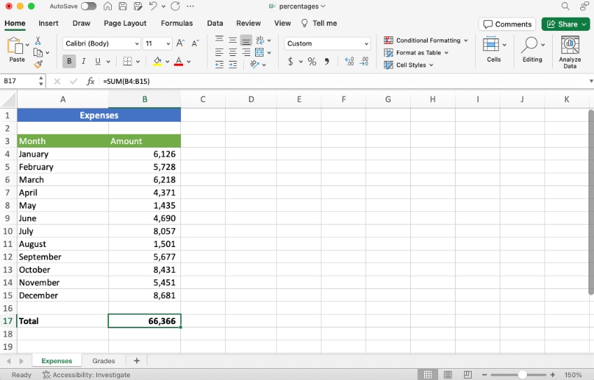
This worksheet is for Expenses. Later in this tutorial, we’ll use the Grades worksheet. Numbers can represent almost anything. But the process for doing a percent change formula Excel doesn’t change.
2. Why Calculate a Percentage Increase?
Let’s say you anticipate that next year’s costs will be 8% higher, so you want to see what they are.
Before writing any percentage formulas in Excel, it’s helpful to know that Excel is flexible. You can type percentages with a percent sign (like 20%) or as a decimal (like 0.2 or just .2). To Excel, the percent symbol is only formatting.
We want to show the total estimated amount, not just the increase.
3. Build a Percent Increase in Excel Formula
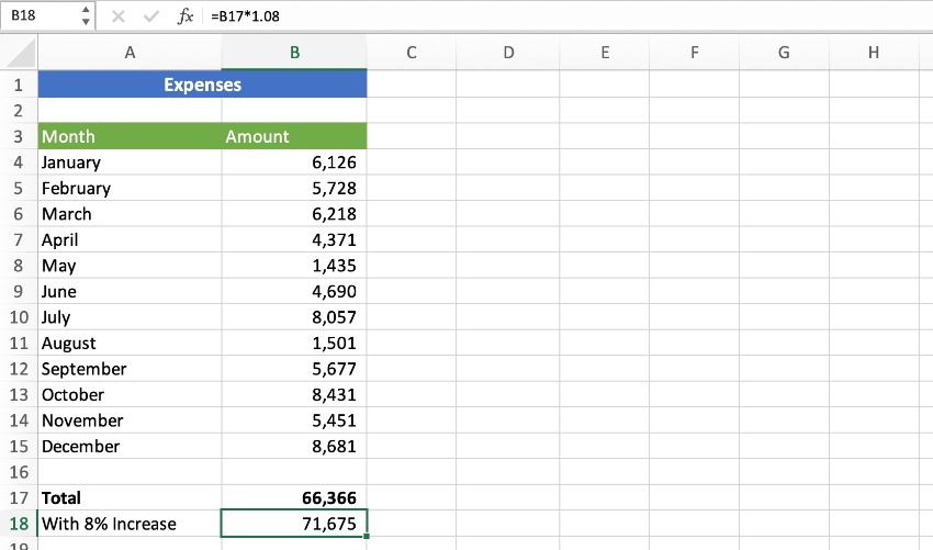
Begin in cell A18. There, type a header reading With 8% Increase. Since this mixes a number with text, Excel will automatically treat the entire cell as text.
Now, press the Tab key to move to the next cell, B18. In B18, enter this Excel percentage formula:
=B17*1.08
You could also type:
=B17 * 108%
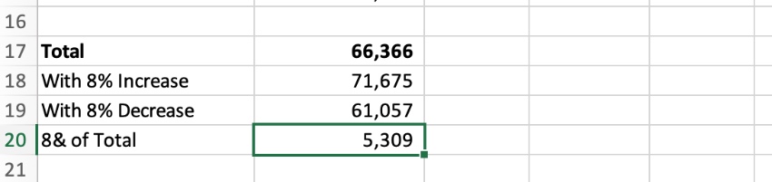
As you can see below, the results display when you hit Enter. The number is 71,675.
4. Build a Decrease Percentage Formula in Excel
Maybe you think your expenses will decrease by 8 percent instead. To see those numbers, the formula is similar. Start by showing the total, lower amount, not just the decrease.
Here's how to make a percent change formula Excel for a decrease.
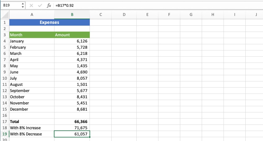
Move to cell A19. In it, type a header reading With 8% Decrease. Then, tab over to cell B19. Enter this Excel percentage formula: =B17*.92. When you hit Enter, the result of 61,057 will appear.
Want more flexibility in changing the percentage up or down? This is a good modeling tool. For this, go to cell B18. Type in =B17 -(B17*0.08) , if you’re measuring a decrease. Use a plus sign if you want to track an increase.
This is the best way for how to calculate a percent increase in Excel!
5. Calculate a Percentage Amount in Excel
Above, we learned how to calculate a percent increase in Excel, along with a decrease. The results were the new total: the original value, adjusted by the amount of the change.
But what if you want to see the percent amount itself, not the new total? For this, we can use a different Excel percentage formula.
In cell A20, keyboard in another header: 8% of Total. Then, tab over to cell B20 and input this formula:
=B17*0.08.
You could also use =B17*8%.
Let's see the result of our percentage formula in Excel. When you hit Enter, the result will be 5,309.
6. Make Adjustments Without Rewriting Formulas
A great way to use a percent change formula in Excel is to model different scenarios.
This involves changing out the percentages for different values to see how they affect overall totals. It’s often useful to be able to change the percentage without having to rewrite any formulas.
To do this, we’ll put the percentage in a cell of its own. This way, it can be changed without altering the percentage formula in Excel. Enter the header text below in cells A22, A23, and A24.
Now, place the percentage in cell B22. We’ll use 8% again. Type that in, and press Enter.
In cells B23 and B24, enter these formulas. The first gives you the total, plus 8%. The other subtracts 8%:
In cell B23:
=B17+B17*B22
In cell B24:
=B17*(100%-B22)
7. Calculate a Percentage Change
You might also want to calculate the percentage change from one month to the next month. That would give you a picture of whether costs were heading up or heading down. So, let’s do that down column C.
The general rule to calculate a percentage change with a percentage formula in Excel:
=(new value - old value) / new value
Since January is the first month, it doesn’t have a percentage change. The first change will be from January to February, and we’ll put this next to February’s number.
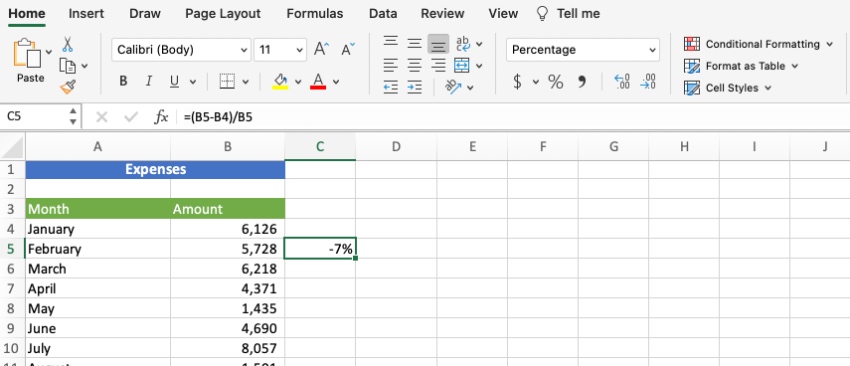
To calculate the first percentage change, enter this percent change formula in C5:
=(B5-B4)/B5
Excel displays this as a decimal, so click the Percent Style button on the ribbon to format it as a percent.
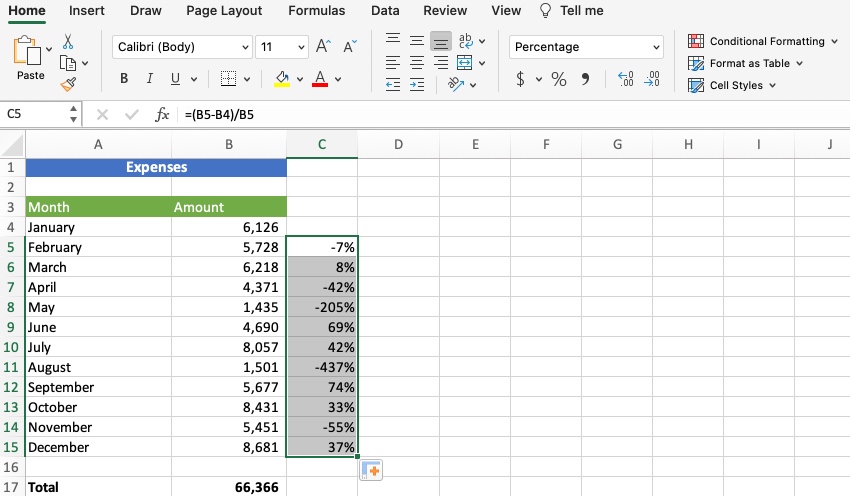
Now that we know what the percent change is from January to February, we can AutoFill the formula. Drag down formulas in column C to show the remaining percent changes for the year.
To do that, roll the mouse pointer over the dot in the lower-right corner of the cell that shows -7%. When the mouse pointer becomes a crosshair, double-click.
Just like that, the formula will copy down to the cells below. The numbers will be selected. You can click Percent Style on the ribbon again to convert them to percentages.
8. Calculate a Percentage of Total
The final technique on this sheet is to find the percent of total for each month. For a percent of total calculation, think of a pie chart where each month is a slice, and all the slices add up to 100%.
Whether with Excel or with pencil and paper, the way to calculate a percentage of total is with a simple division:
Component number/total
… and format it as a percentage.
In this example, we divide each month by the total at the bottom of column B.
Click on C3 and AutoFill one cell across to D3. Change D3 to read % of Total.
In D4, type this formula, but don’t press Enter just yet:
=B4/B17
Before entering the formula, we want to be sure of preventing AutoFill errors. Since we’re going to AutoFill down the column, the denominator, which is now B17, shouldn’t change. If it does, the numbers for February through December will be wrong.
Make sure the text cursor is still in the formula, on the “B17” denominator. Press the F4 key (on Mac, press Fn-F4).
That inserts dollar signs before the column and the row, turning the denominator into $B$17. The $B means that column B won’t increase to column C, etc. and the $17 means the row won’t increase to $18, etc.
Make sure your formula reads:
=B4/$B$17
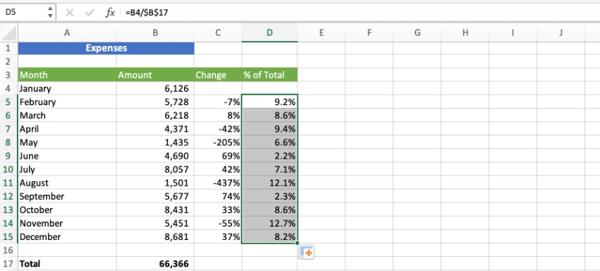
Now, you can press Enter. Then, apply the Percent Style. And finally, you can AutoFill downward to view the % of Total for each line item. It’s amazingly easy!
9. Percentage Ranking
Ranking numbers by percent is a statistical technique. You’re probably familiar with it from school. You and your classmates have grade point averages, so each of you is ranked in a percentile. The higher your grades, the higher your percentile.
The list of numbers (grades, in this example) are in a range of cells that Excel calls an array. There’s nothing special about an array and you don’t have to define it. That’s just what Excel calls the range of cells you plug into a formula.
Excel has two functions for percentage ranking. One function includes the beginning and ending numbers of the array. The other function doesn’t.
Look at the second tab in the worksheet: Grades.
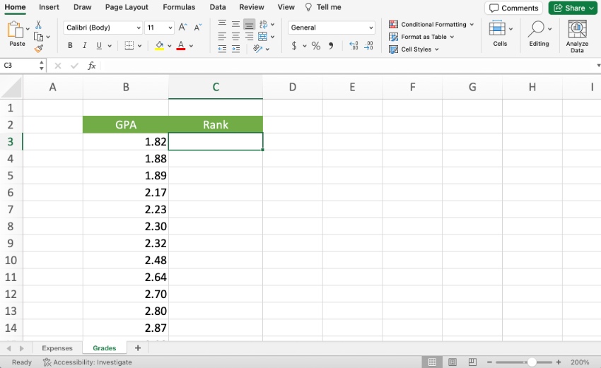
This shows a list of 35 grade point averages, sorted in ascending order. The first thing we want to do is find the percentile rank for each one. To do this, we’ll use the =PERCENTRANK.INC function. The “INC” part of that function means “inclusive," as it'll include the first and last grades in the list.
To exclude the first and last numbers in the array, you would use the =PERCENTRANK.EXC function.
The function takes two mandatory arguments, and the syntax is: =PERCENTRANK.INC(array, entry)
- array is the range of cells that contains the list (in this example, it’s B3:B37)
- entry is any number or cell in the list
Click C3, the first one in the list. Start typing this formula, but don’t press Enter, yet:
=PERCENTRANK.INC(B3:B37
This range needs to be an absolute reference so we can AutoFill to the bottom.
Press F4 (on the Mac, press Fn-F4) to insert dollar signs.
The formula should now look like this:
=PERCENTRANK.INC($B$3:$B$37
In each case down column C, we want to know the percent rank of the entry in column B.
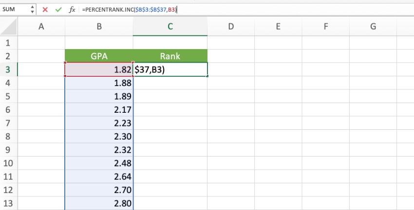
Click B3, then close the parenthesis.
The formula is now this: =PERCENTRANK.INC($B$3:$B$37,B3)
Now we can fill in and format the numbers.
If necessary, click back on C3 to select it. Double-click the AutoFill dot on C3. That automatically fills down the column.
On the ribbon, click the Percent Style button to format the column as percentages. You should now see the finished result:
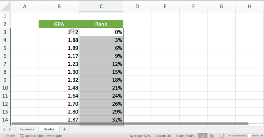
So, if you had very good grades and your GPA was 3.98, you would say that you ranked in the 94th percentile.
10. Finding the Percentile
You can also find the percentile directly, using the PERCENTILE functions. With these functions, you enter a percent rank, and it'll return a number from the array that corresponds to that rank. What if the exact number you want isn’t listed? Excel will interpolate the result and return the number that “should” be there.
When would you use this? Let’s say you plan on applying for a graduate program. That program accepts only students who score in the 60th percentile or higher. So, you want to know what GPA is exactly 60%. Looking at this list, we can see 3.22 is at 59% and 3.25 is at 62%, so we can use the =PERCENTILE.INC function to find the answer.
The syntax is:
=PERCENTILE.INC(array, percent rank)
- array is the range of cells that contains the list (same as the previous example, B3:B37)
- rank is a percentage (or a decimal between and including 0 and 1)
Just like with the percent ranking functions, you could use =PERCENTILE.EXC to exclude the first and last entries in the array. But that’s not what we want in this example.
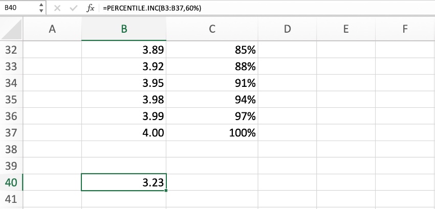
Click on B39, right below the list. Then, enter this formula:
=PERCENTILE.INC(B3:B37,60%)
Since we aren’t going to AutoFill this formula, there is no need to make the array an absolute reference.
On the ribbon, click the Decrease Decimal button once, to round the number to two decimal places.
The result is that in this array, a 3.23 GPA is the 60th percentile. Now you know the grades you need for acceptance into the program.
Learn More About Microsoft Excel (Tips and Tricks for 2024)
In this tutorial, you learned how to calculate percentage in Excel. Plus, we explored a formula for percentage increase in Excel. Percent increase in Excel formulas are easy with the approach you just learned, and you'll never make a mistaken calculation!
It’s only one of the countless features that Excel includes to help you manage data better. Here are more helpful tutorials to elevate your Excel skills in moments:
 How to Create an Invoice in Excel Using a Template
 How to Embed (& Automatically Link) Excel Files in Word
 How to Embed Excel Files and Link Data Into PowerPoint
 What Is Excel Art? & How to Start Making Your Own (Pixel Art Guide)
The Best Source for the Top Microsoft Excel Templates (With Unlimited Downloads)
The best way to save time in Microsoft Excel is to use pre-built templates. These templates take care of graphic design work for you. All you've got to do is fill in your own data.
The top source for these templates is Envato Elements. Elements has a variety of premium Microsoft Excel templates available now. Use them for invoices, lists, and more.
And that’s not all. Elements includes millions of digital assets in total! These include:
- fonts
- music
- stock photos
- and countless other categories
The Elements offer is powerful: unlimited downloads. For a flat monthly rate, you can download and use as many of these templates and assets as you want! This gives you unmatched flexibility as a creative. And with AI-powered search, you can find anything you need in seconds.
Choose a premium template from Envato Elements and you’ll enjoy:
- Easy-to-use layouts. Not a graphic designer? No need. Templates are built by experts to always help your data look its best.
- Time savings. All you do is fill in your data. Complex formula work and more has already been handled for you.
- Inspiring designs. Wondering how best to present your data in spreadsheet form? These templates have plenty of ideas inside.
As you can see, Envato Elements is the ultimate creative value in 2024 and beyond. Join today and start exploring.
Put a Percentage Formula in Excel to Work Today
In this tutorial, you learned how to work with a formula for percentage increase in Excel. As you think of how to use Excel percentage formula options, the key is to streamline your workflow. How can you put Excel formulas to work for you?
Any time you work with data, you can use a percentage formula in Excel. Think of it as the ultimate way to work more efficiently. The percent change formula Excel technique does the work for you.
With ease, you can visualize scenarios and analyze data that you already have. It’s a key part of the journey to becoming an Excel expert. So, what are you waiting for? Choose an Excel template from Envato Elements. Then, get started today!
Editor's Note: This tutorial was first published in June 2016. It's been completely reviewed and revised for accuracy by Andrew Childress.
 By
By